Megan Langford

Examining the Activity of Quadratic Equations in the xb Plane

Let us first consider the basic quadratic equation

When graphing in relation to the xb plane, we get:

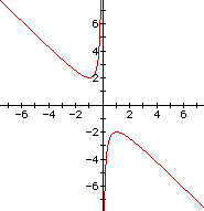
This graph displays the relationship between the x and b values. It is important to note the activity for several different areas of the graph. First, as x increases over the interval (-¥,1), the b value decreases. Then right around x=-1, the curve changes direction as the b value abruptly increases. There seems to be no value at x=0, which makes sense because when you plug 0 in for x in the equation, you end up with 1=0. This of course does not make sense. Also, as x increases over the interval (0,1), the b value is also increasing. But again near x=1, the curve changes direction again and b decreases as x increases. Finally, we can also notice that there is a substantial gap on the graph located between the curves. So we see that there appears to be no behavior for the graph where b is between -2 and 2. To explain this behavior, let’s take a look at the behavior of the roots of the equation.

With each point along the curves, the b values correspond to a root of the given quadratic equation. We can verify this by plugging both b and x values for each point into the equation to check.

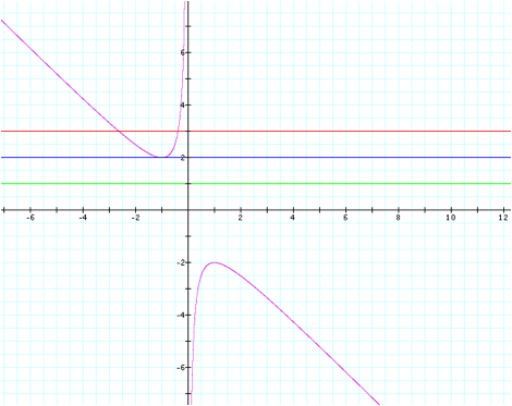
By showing the graph of the equation b=3, we are giving just one example of the behavior of the original function with any horizontal line where b is greater than 2. As we can see in this case, the line b=3 intersects with the function at exactly two points. As it turns out, when we algebraically solve for x at the given b value, we come up with two real root solutions which form the x coordinates for the points of intersection. Using the Quadratic Formula, we can solve for the x values:

So we see that this is equivalent to approximately -.38197 and -2.61803. If we look at the graph where the pink and red lines intersect, the b values do appear to be near these two numbers, so we know that this is correct.

However, we can also notice that when b=2, this line touches the graph at only one point. We can investigate the cause of this behavior by solving for x when b=2.

Working out the algebra behind this situation shows us that the reason for this oddity is because when b=2, solving the equation for x gives us a duplicate of the same answer. Since the bottom curve has the same behavior as the top one, we can see that we would get another duplicate answer of x=1 if we were to solve for x when b=-2.

Finally, since we have a gap on the graph for all b values between -2 and 2, there are no points of intersection for the original function and b=1. To take a look at why this is the case, we can again solve for x when b=1.

Since we all know that is an imaginary number, there is no real solution to the value of x when b=1. Again, since the bottom curve has the same shape as the top one, we can see that if we were to solve for x when b=-1, we could get another imaginary number and hence, no real solution.

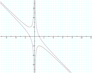
This graph shows us the relationship between the number of roots and the number of intersection points between the red and pink equations. Since the line where b=3 crosses the graph at exactly two points, we have two real roots. Along the line where b=2, it touches the original function at exactly one point, so we have one real root. Clearly, the line where b=1 never crosses the original function, so there are no real roots at that value. We could mirror this same graph using b=-1, -2, and -3, and we would find the same results that we have found for the positive b values in this graph. Also, since the graph continues in the same pattern, it will have exactly two real roots where b is greater than 2 or less than -2.

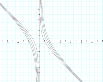
To examine one more effect of a change to the function, let us take a look at the difference in graphs as we change the c term of the equation. For comparison’s sake, let us set c=-1 and compare with our original graph.

We can now determine that a change in the c term does have a rather significant impact on the overall shape of the graph. One main difference is that no matter where you place a horizontal line on this new function’s graph, there will always be two roots. This can be explained again by algebraic reasoning to show that:

So regardless of the b value, there will always be a two roots to solve the equation. In fact, we can further investigate that this will be the case for any value of c<0. Let’s take a look.

Hence, we can see that this trend will continue that for all values of c<0, we will continue to have two real solutions for the x value.